Do you have a data-heavy spreadsheet, making it difficult to see the data you need to analyse? Instead of moving the taskbar continuously or deleting the rows, you can hide the columns, analyse the data, then unhide them.
The possibility to hide and unhide columns in Excel helps conceal some columns using this feature. Microsoft Excel makes it easy to hide or unhide rows and columns more efficiently. In this article, you will learn how to hide and unhide columns in Excel.
Remember, the best way to protect the worksheet is to lock it with a password.
Why Would You Hide Columns in Excel?
There are a lot of reasons to hide columns in Excel. For instance:
- While comparing non-adjacent columns, you can hide the in-between columns to make them appear side by side.
- Hide helper columns to conceal those containing formulas that might confuse other users.
- Hide columns that contain private or sensitive data, such as salary, age, and other important information.
How Do You Hide Columns in Excel?
There are different ways you can hide and unhide a column in Excel. Let’s look at each of them. To better understand the process, we will use the following example: an Excel sheet containing details of a trust that collects money from donors to help a local community.
This worksheet contains donor names, IDs, periodicity of donations – such as monthly, quarterly, or annual donation amounts – and their contact information. The columns that contain donation numbers and contact information do not need to be visible and can be hidden.
Method 1: Using a Context Menu
- Select the column you wish to hide from other users by clicking the column header,
- Right-click on the selected column,
- On the menu, select the Hide option,
- Now the selected column is hidden.
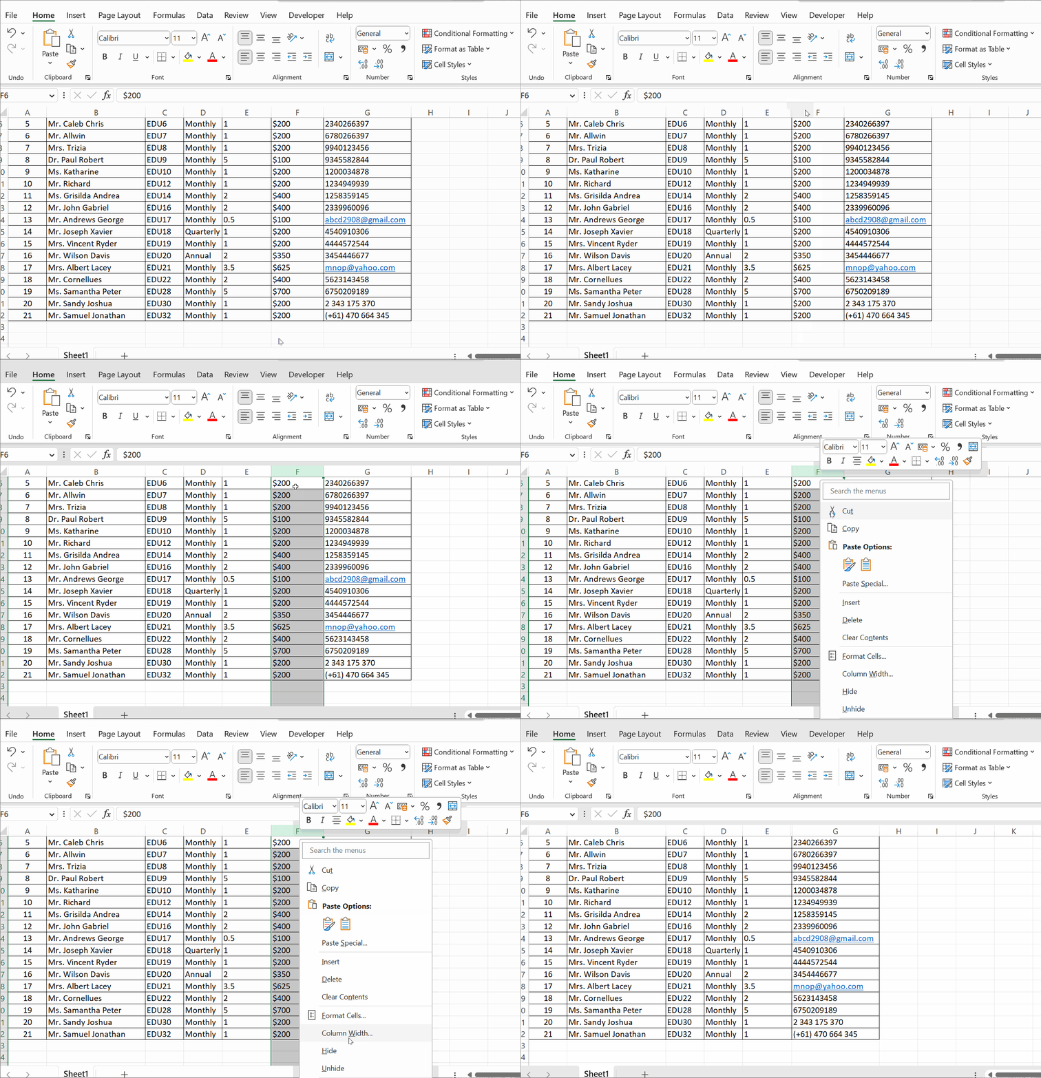
Hide a column using the context menu.
In the above example, we hide column F as it contains the amount donated by each donor. To hide it, select column F by clicking on the column header, right-click, and select the option Hide.
After we hide column F, you can see that it is hidden between columns E and G, but there is a small line between E and G.
Method 2: Using the Ribbon
- Select the column you wish to hide from other users by clicking the column header.
- Go to Home →Format (in the Cells group).
- In the Visibility section, hover over the Hide & Unhide option and choose Hide Columns.
- The selected column is hidden.
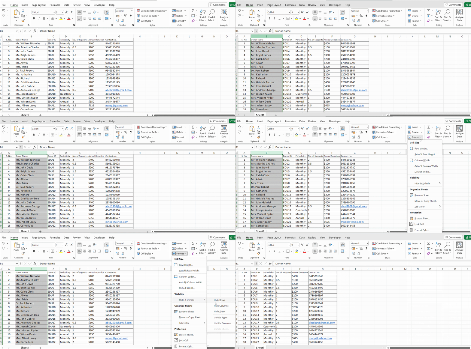
Hide a column using a ribbon.
Method 3: Using Shortcut
- Select the desired column, and use the shortcut by pressing the keyboard keys Ctrl+0 (zero).
- Select a cell within a single column, and use the shortcut key Ctrl+0 (zero) to hide a single column.
- To hide non-adjacent columns, select a column, then hold the Ctrl while clicking on additional columns that are non-adjacent to select them. Then, press Ctrl+0 (zero).
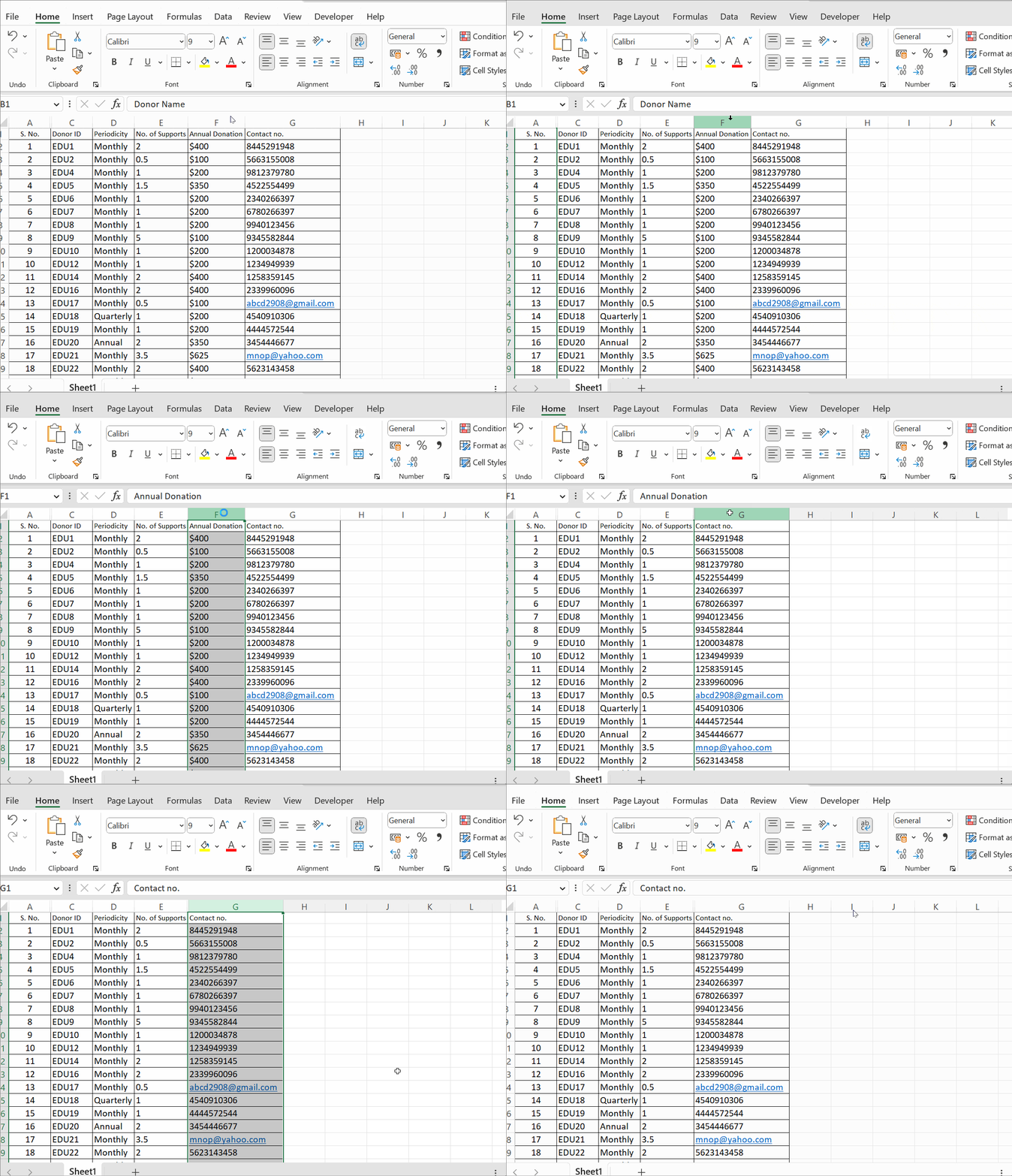
Hide a column using the shortcut key.
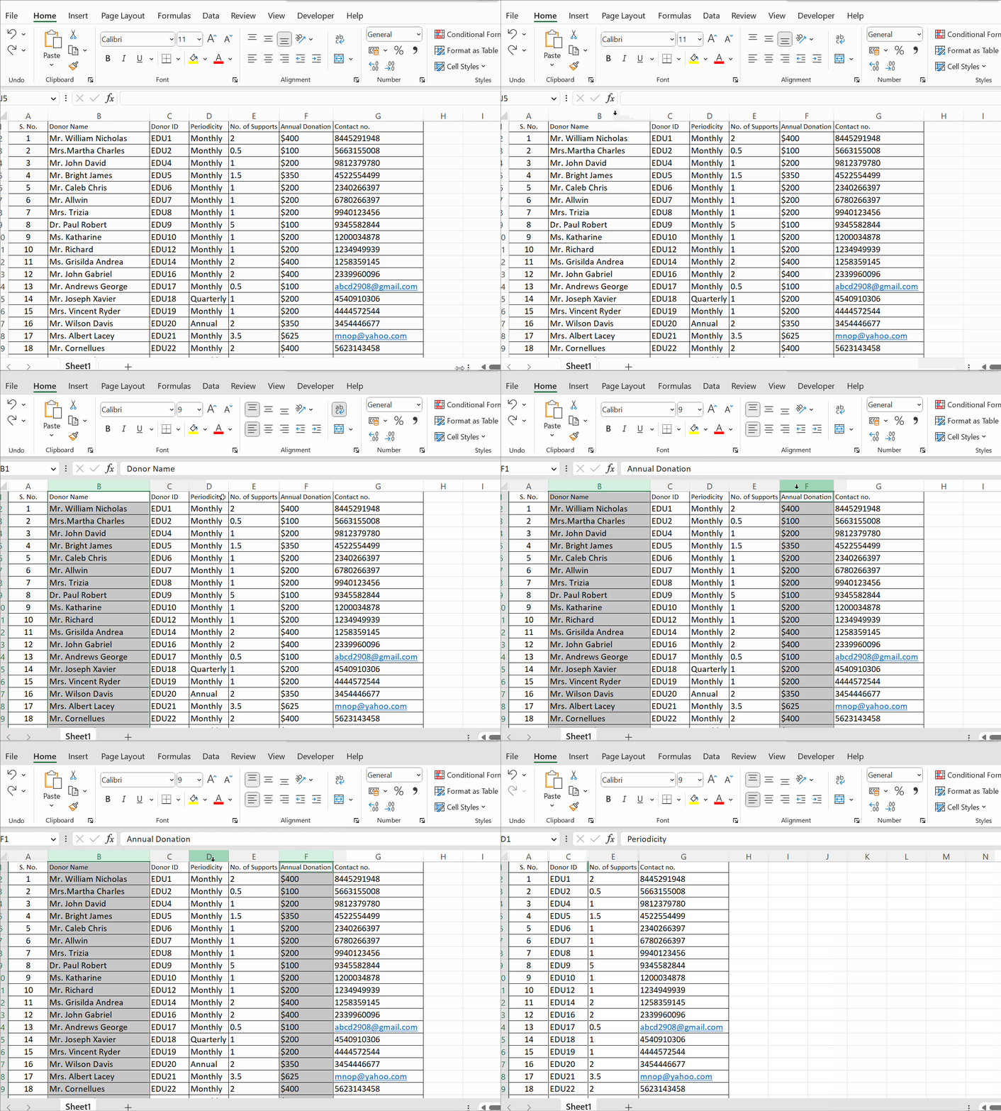
Multiple non-adjacent columns are selected and hidden using the shortcut key, Ctrl+0.
Note: If the selected column does not hide when you press Ctrl+0 (zero), follow these steps to activate the shortcut keys.
- Select Time & Language → Typing → Advanced Keyboard Settings → Input Language hotkeys.
- In the open window, choose the tab Advanced Key Settings → Change Key Sequence for Between Input Languages to ‘Not Assigned.’
Method 4: By Grouping
When you find that the worksheet has numerous columns and a few adjacent columns have to be hidden, you can group them. Follow these steps to group and then hide them.
- Select the columns that you wish to hide.
- Go to Data → Outline → Group.
- Select Group. You can find this line on top of the columns you grouped, along with the ‘-’ sign.

- Click the ‘-’ sign, and the columns should be hidden.
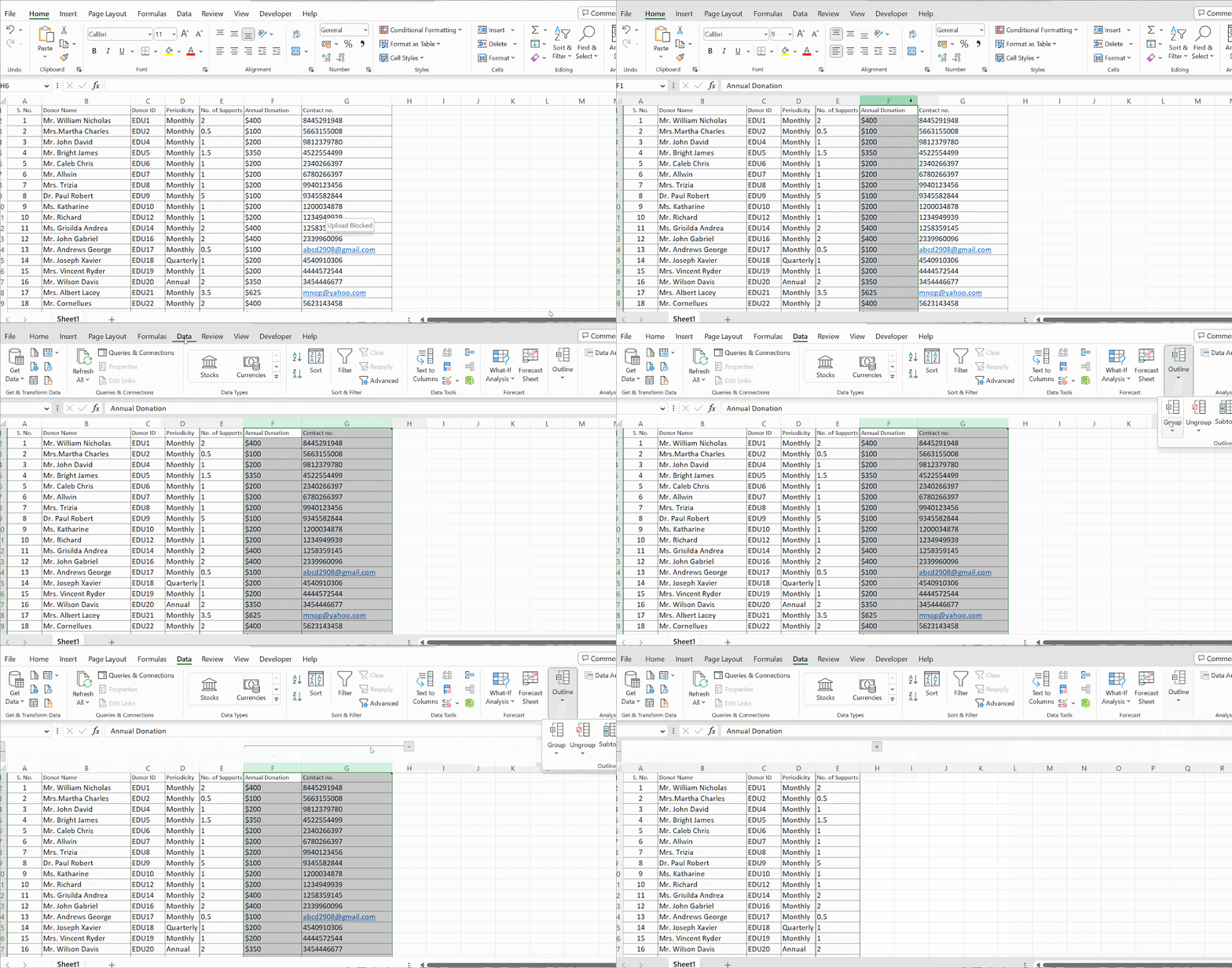
Hide more columns by grouping.
Method 5: Hide Unused Cells
You can hide all blank cells to the right of the table to make the working area of your sheet visible. The steps to do this are:
- Select a cell, then press Ctrl+Shift+Right Arrow to highlight the blank cells until the end of the sheet.
- Press the shortcut key Ctrl+0 (zero) to hide the selected cells.
- The worksheet will only show your table.
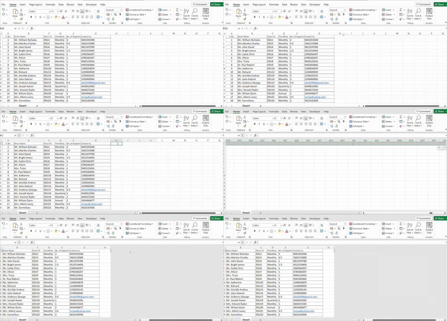
Hide unused columns.
How Do You Unhide Columns in Excel?
You can restore the hidden column in the following ways.
Method 1: Unhide Using the Context Menu
- Click on any of the cells in the worksheet that contain a hidden column.
- Then, right-click on it to display the context menu.
- Select Unhide option.
- The hidden column is now restored.
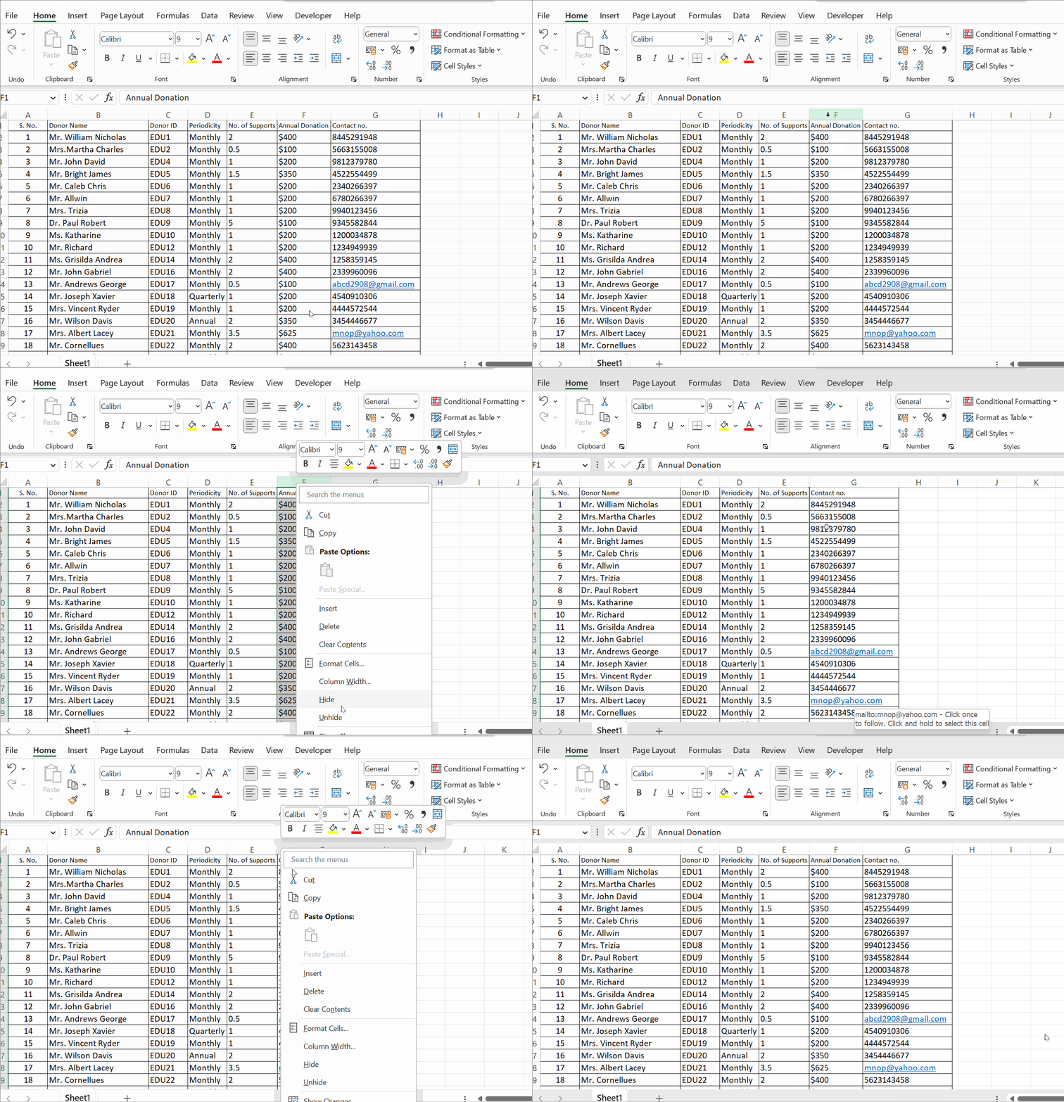
Unhide a column using the context menu.
Method 2: Unhide Using the Ribbon
- Select the entire worksheet by pressing the button on the top left corner to unhide all the hidden columns in the worksheet.

Select all buttons at the top left corner of the worksheet.
- All columns are now selected.
- Now, select Home → Format → Hide & Unhide → Unhide Columns.
- The hidden columns are now restored.
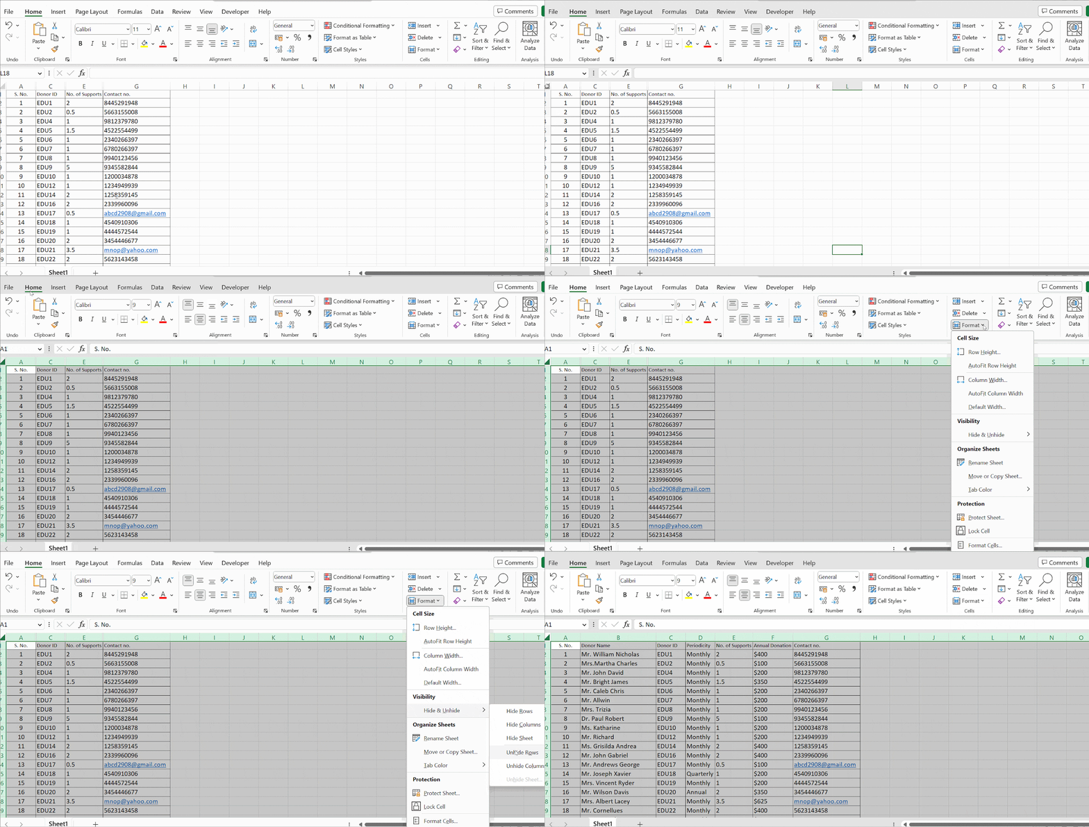
Unhide a column using a ribbon.
Method 3: Using the Shortcut Key To Unhide Columns
To unhide the hidden columns, highlight at least one cell in the columns on both sides of the hidden column and press the shortcut key Ctrl+Shift+0 (zero).
Note: This key combination won’t work for some versions of Windows.
Method 4: Unhide By Ungrouping
- When you hide columns by grouping, you must ungroup those columns to unhide them.
- Simply click on the ‘+’ sign to restore the hidden columns.

Unhide by ungrouping
Note: Even after you unhide by ungrouping, you may find a single line above the columns to indicate that columns were grouped.
To make that line disappear, click Data → Outline → Ungroup.
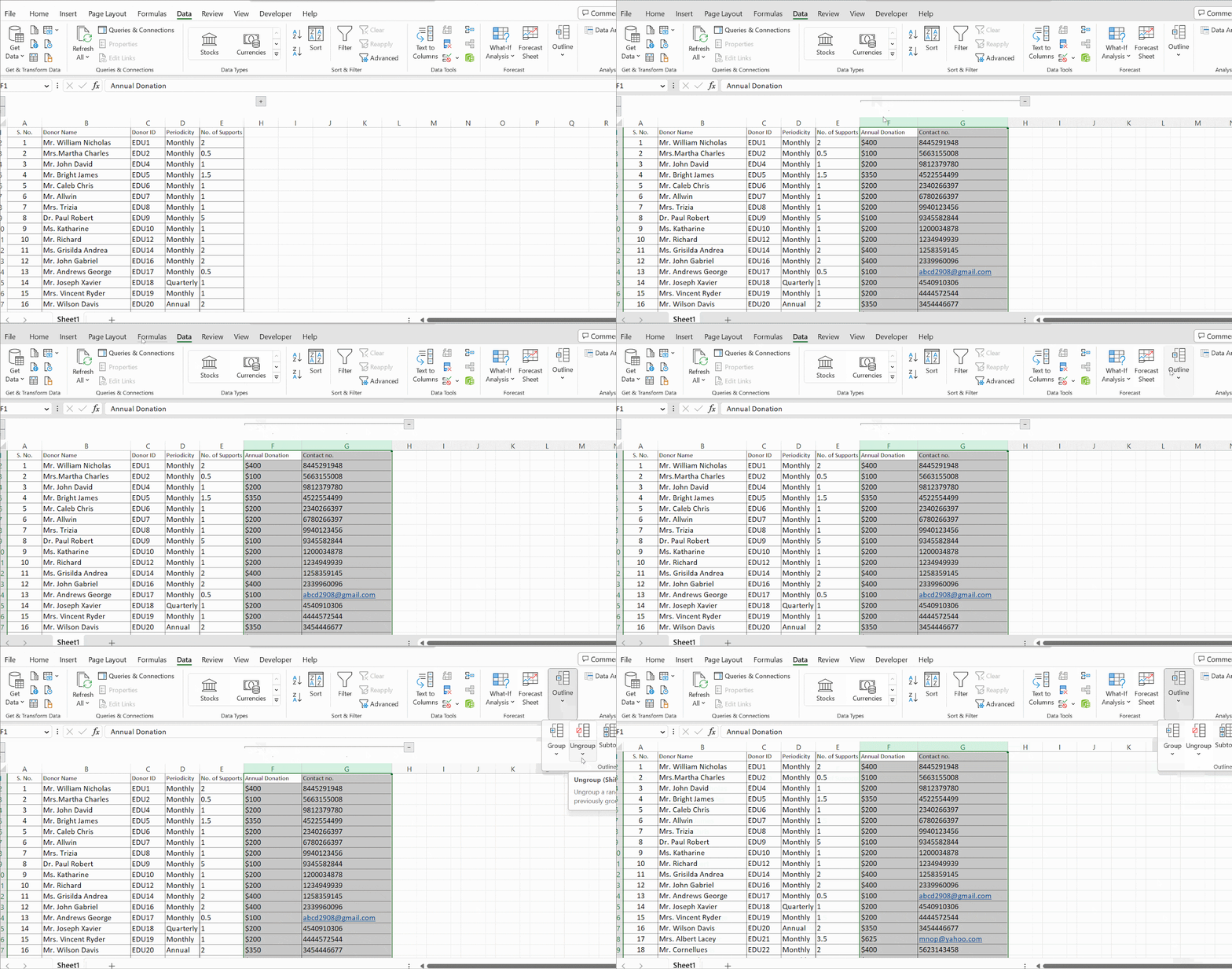
Ungroup columns
Method 5: Unhide Using the Go-To Option
- Though the column is hidden and not visible, you can select and unhide the first cell.
- Select Home → Find & Select → Go To.
- Enter the cell reference, B1, which selects the hidden cell.
- Then select Home → Format → Hide & Unhide → Unhide Columns.
- The hidden columns are now restored.
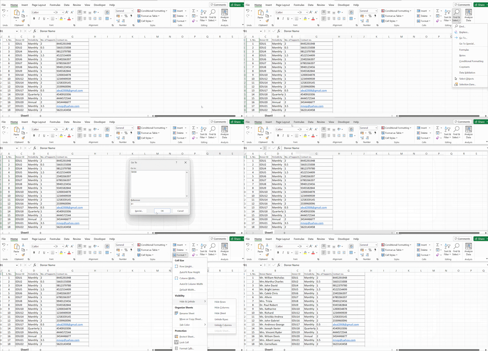
Unhide using the ‘Go-To’ option.
FAQs
How Do You Hide and Unhide Columns Easily?
Select the columns that you want to hide. If they are non-adjacent columns, press Ctrl to select them. Right-click on one of the selected columns and then right-click on it and select the Hide option. You can unhide them by selecting the column, right-clicking on it and selecting the Unhide option.
How Do You Hide and Unhide Rows in Excel?
Select a row or rows that you wish to hide. If they are non-adjacent rows, select them by pressing Ctrl and clicking on the specific row. Right-click on it, and from the menu, select the option Hide. To unhide a row, select all the cells, and go to Home → Format → Hide & Unhide → Unhide Columns.
Final Thoughts
Microsoft Excel is an excellent tool for storing, sorting, and organizing data. While organizing your sheet, you may find it helpful hiding specific columns that you may not be using or don’t wish others to see, but you also don’t want to delete either.
Certification in Excel can give you a competitive edge, whether you are a job seeker or a professional.
Learning more Microsoft Office Excel functions is vital for succeeding in the current workplace. To help, check out our article, “The Top 5 Excel Functions to Make Work Easier,” and master new skills in Excel.
You can also check out Pitman Training’s Microsoft Excel Courses and Certificate and jumpstart your career by learning more about Excel functions and formulas. You can also visit our website and get your certification in Microsoft Office and Microsoft Word.


